13 min to read
Bayesian Network with Python
I wanted to try out some Python packages for modeling bayesian networks. In this post, I will show a simple tutorial using 2 packages: pgmpy and pomegranate.
Why use Bayesian networks?
Bayesian networks are useful for modeling multi-variates systems. Suppose you have a random system with $N$ random variates, namely $X_1, \dots, X_N$. If you know the total joint cumulative distribution function (CDF), that is $F(X_1, \dots, X_N)$, then you can theoretically compute any partial distribution, and you likely won’t need a bayesian network. But, in practice, we generally do not know $F(X_1, \dots, X_N)$ and we need to estimate it somehow. Because of the curse of dimensionality, fitting $F$ is exponentially difficult and requires a lot of data.
Using bayesian network helps simplify the system and give a structure of interactions between the $N$ variates. The network is a graph with $N$ node (one for each variate), and the arcs define the causality betweens the variates. For example, the arc (age, salary) means that salary depends on the age. A bayesian network must a acyclic graph, that is, no loop.
We want to find the distribution $F_i = F(X_i | X^i_1, \dots, X^i_{n(i)})$ of each node $i$ conditional to the $n(i)$ parent nodes $X^i_1, \dots, X^i_{n(i)}$. If every node has few parents (i.e., $n(i)$ is small), then it is much easier to fit the $F_i$’s than $F(X_1, \dots, X_N)$.
Bayes’ law
If the name isn’t obvious enough, Bayes’ law is at the heart of the bayesian network model. This law is derived directly from the law of conditional probabilities. If we have random variate $X_1$ and $X_2$ then \[ F(X_1, X_2) = F_1(X_1 | X_2)F_2(X_2) = F_2(X_2 | X_1)F_1(X_1). \] By switch one the multiply to the other side: \[ F_1(X_1 | X_2) = \frac{F_2(X_2 | X_1)F_1(X_1)}{F_2(X_2)}. \]
Note that we can replace the CDF functions $F$ by a probability mass $P$.
Causality? Yes or No?
One important thing to be aware is that Bayes’ law and bayesian networks do not prove causality! They exploit the conditional distributions and the dependence (or independence) of the variates. For example, you may have variables Age and Salary that are correlated. Without a larger context, you can model $Age \rightarrow Salary$ or $Salary \rightarrow Age$. Nothing proves that one causes the other. In reality, many things are correlated without causality, like the values of a person’s house and car, for example.
The causality implied by the bayesian network graph is a choice from the modeler. Unless the user knows all the rules affecting the system including the probability distributions, there are generally more than one way to construct the network graph.
The Monty Hall problem
This problem is based on a game show hosted by Monty Hall. Here’s how the game works:
- A prize is hidden between one of 3 doors (A, B and C).
- The guest picks one door.
- Among the 2 remaining doors, Monty opens one door without the prize.
- The guest is asked if he wants to switch doors.
The question is: “Would you switch doors or not?”
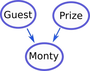
We will use a bayesian network to determine the optimal strategy. The graph model is displayed below. The initial choice of the guest and location of the prize are independent and random. However, Monty’s choice depends on both the choice of the guest and the location of the prize.
Package: pgmpy
Let’s try to solve this using pgmpy. You can install this package with
pip install pgmpy
Let’s build the network:
from pgmpy.models import BayesianModel
from pgmpy.factors.discrete import TabularCPD

model = BayesianModel([('Guest', 'Monty'),
                       ('Prize', 'Monty')])
state_names = {'Guest':['A','B','C'],
               'Prize':['A','B','C'],
               'Monty':['A','B','C']}

# define the conditional probabilities
cpd_guest = TabularCPD(variable='Guest', variable_card=3,
          state_names=state_names,
          values=[[1/3],
                  [1/3],
                  [1/3]])
cpd_prize = TabularCPD(variable='Prize', variable_card=3,
          state_names=state_names,
          values=[[1/3],
                  [1/3],
                  [1/3]])

cpd_monty = TabularCPD(variable='Monty', variable_card=3,
          state_names=state_names,
          values=[[0.0, 0.0, 0.0,  0.0, 0.5, 1.0,  0.0, 1.0, 0.5],
                  [0.5, 0.0, 1.0,  0.0, 0.0, 0.0,  1.0, 0.0, 0.5],
                  [0.5, 1.0, 0.0,  1.0, 0.5, 0.0,  0.0, 0.0, 0.0]],
          evidence=['Guest', 'Prize'],
          evidence_card=[3, 3])

# add the probabilities
model.add_cpds(cpd_guest, cpd_prize, cpd_monty)
model.check_model()
Let’s do some predictions.
Suppose the guest chose door A and Monty opened door B.
We use the function predict_probability to predict
the location of the prize.
# use Pandas dataframe for inputs
import pandas as pd

observed = pd.DataFrame(data={'Guest':['A'],'Monty':['B']})
model.predict_probability(data=observed)| Prize_A | Prize_B | Prize_C | |
|---|---|---|---|
| 0 | 0.333333 | 0.0 | 0.666667 |
The bayesian network predicts 2/3 chance that the prize is behind door C. So the guest should switch doors!
If Monty opened door C instead of door B, the guest should still switch doors.
observed = pd.DataFrame(data={'Guest':['A'],'Monty':['C']})
model.predict_probability(data=observed)| Prize_A | Prize_B | Prize_C | |
|---|---|---|---|
| 0 | 0.333333 | 0.666667 | 0.0 |
Why is switching optimal?
Why is the probability to win higher by choosing the other door? The key is that Monty knows which door hides the prize. His choice may contain information (is dependent) on the location of the prize. If the guest chose door A, and Monty chooses door B instead of door C, it could be for a good reason (the prize is behind door C).
It is explained nicely in this Youtube video. Suppose the game has 100 doors, instead of 3. The guest picks 1 door. Then, Monty opens knowingly 98 non-winning doors, and leaves 1 door closed. Which door has the higher chance to have the prize? The other door.
Package: pomegranate
Let’s now try to model the same bayesian network with the package pomegranate. The following code is taken from their tutorial.
Note: I installed this package with anaconda, because it failed to compile with pip.
Let’s define the probability distributions and create the network model.
from pomegranate import *

Guest = DiscreteDistribution({'A':1/3, 'B':1/3, 'C':1/3})
Prize = DiscreteDistribution({'A':1/3, 'B':1/3, 'C':1/3})
Monty = ConditionalProbabilityTable(
        [['A', 'A', 'A', 0.0],
         ['A', 'A', 'B', 0.5],
         ['A', 'A', 'C', 0.5],
         ['A', 'B', 'A', 0.0],
         ['A', 'B', 'B', 0.0],
         ['A', 'B', 'C', 1.0],
         ['A', 'C', 'A', 0.0],
         ['A', 'C', 'B', 1.0],
         ['A', 'C', 'C', 0.0],
         ['B', 'A', 'A', 0.0],
         ['B', 'A', 'B', 0.0],
         ['B', 'A', 'C', 1.0],
         ['B', 'B', 'A', 0.5],
         ['B', 'B', 'B', 0.0],
         ['B', 'B', 'C', 0.5],
         ['B', 'C', 'A', 1.0],
         ['B', 'C', 'B', 0.0],
         ['B', 'C', 'C', 0.0],
         ['C', 'A', 'A', 0.0],
         ['C', 'A', 'B', 1.0],
         ['C', 'A', 'C', 0.0],
         ['C', 'B', 'A', 1.0],
         ['C', 'B', 'B', 0.0],
         ['C', 'B', 'C', 0.0],
         ['C', 'C', 'A', 0.5],
         ['C', 'C', 'B', 0.5],
         ['C', 'C', 'C', 0.0]], [Guest, Prize])

s1 = Node(Guest, name="Guest")
s2 = Node(Prize, name="Prize")
s3 = Node(Monty, name="Monty")

model = BayesianNetwork("Monty Hall Problem")
model.add_states(s1,s2,s3)

model.add_edge(s1, s3)
model.add_edge(s2, s3)
model.bake()
Suppose the guest chose door A and Monty chose B. Let’s get a prediction on the location of the prize. With pomegranate, we don’t need to use pandas’ DataFrame for input.
model.predict_proba([['A',None,'B']])Again, there is a 66.7% chance that the prize is behind the other door and the guest should switch.
[array(['A',
        {
     "class" :"Distribution",
     "dtype" :"str",
     "name" :"DiscreteDistribution",
     "parameters" :[
         {
             "A" :0.3333333333333334,
             "B" :0.0,
             "C" :0.6666666666666664
         }
     ],
     "frozen" :false
 },
        'B'], dtype=object)]
Alternative version: Monty has no clue
In the original Monty Hall problem, the reason the guest should switch doors is because Monty knows where the prize is.
In this section, let’s consider an alternative game and change the rules such that Monty has no idea which door hold the prize. After the guest chooses a door, Monty will pick randomly one of the 2 remaining doors. If Monty finds the prize, the guest loses.
We will modify the code using the pgmpy package.
We update the conditional probability distribution for Monty’s choice
to reflect that he has a 50%-50% chance of choosing each of the remaining doors.
model = BayesianModel([('Guest', 'Monty'),
                       ('Prize', 'Monty')])

cpd_guest = TabularCPD(variable='Guest', variable_card=3,
         state_names=state_names,
         values=[[1/3],
                 [1/3],
                 [1/3]])
cpd_prize = TabularCPD(variable='Prize', variable_card=3,
         state_names=state_names,
         values=[[1/3],
                 [1/3],
                 [1/3]])

cpd_monty2 = TabularCPD(variable='Monty', variable_card=3,state_names=state_names,
          values=[[0.0, 0.0, 0.0,  0.5, 0.5, 0.5,  0.5, 0.5, 0.5],
                  [0.5, 0.5, 0.5,  0.0, 0.0, 0.0,  0.5, 0.5, 0.5],
                  [0.5, 0.5, 0.5,  0.5, 0.5, 0.5,  0.0, 0.0, 0.0]],
          evidence=['Guest', 'Prize'],
          evidence_card=[3, 3])

model.add_cpds(cpd_guest, cpd_prize, cpd_monty2)
Suppose the guest chose door A and Monty chose door B. Where is the prize?
import pandas as pd

observed = pd.DataFrame(data={'Guest':['A'],'Monty':['B']})
model.predict_probability(data=observed)| Prize_A | Prize_B | Prize_C | |
|---|---|---|---|
| 0 | 0.333333 | 0.333333 | 0.333333 |
This time the result is quite different from the original version of the game. The location of the prize remains uniform with 1/3 chance of being behind each door. It means that, if Monty does not find the prize, switching doors or not has equal chance of winning.